ui <- page_sidebar(title = "My Shiny app",
                   theme = bs_theme(preset = "flatly"),
...)7 Theming and customization
While the default style of a Shiny app out-of-the-box looks much better than its predecessors when Shiny was first developed, it still very much looks quite plain and uninspired. To format the aesthetics of apps to better match a particular organization’s color palette, or to simply make it look more professional, we should take a little extra time to customize the look and feel of our Shiny apps. Below, I will share some examples of ways that we can customize the theme, whether using presets or by selecting colors and styles on your own.

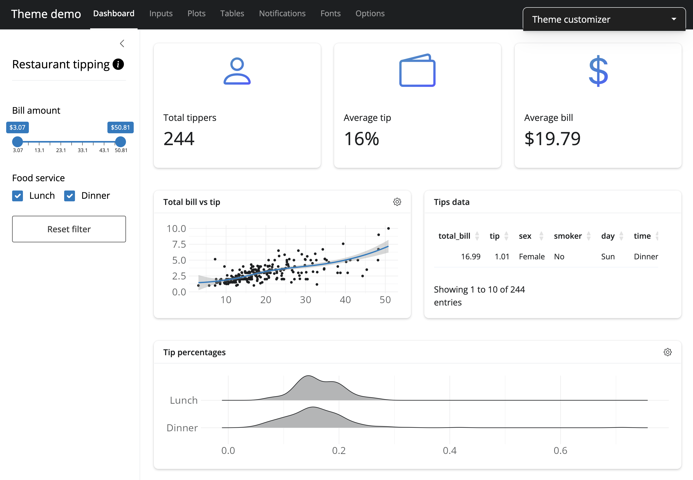
The preset themes that are available through {bslib} come from Bootswatch, which currently includes 25 different light and dark themes. These can be applied as simply as using the bs_theme() function from {bslib}, as shown in the code below:
This ‘flatly’ theme would produce an app that looks like the screenshot example below:

These themes can be explored using a built-in Shiny app from {bslib} using the bs_theme_preview() function, which includes a dropdown panel for customizing different aesthetics for the app. Additionally, these themes can be dynamically explored for your own Shiny app by adding bs_themer() to the server component of your app:
server <- function(input, output, session) {

  # {bslib} widget to explore Bootswatch themes
  bs_themer()

  ...
}
If wanting finer control over the colors, fonts, and font sizes, you can still achieve all of this using the bs_theme() function as opposed to needing to use CSS code directly. In place of specifying a Bootswatch preset, you would need to provide values for different components such as the background (bg) and foreground (fg) colors, accent colors (primary, secondary, success, warning, etc), as well as fonts (base, heading, code) that are either already available on your computer or that are available on Google Fonts (using font_google()). An example of these custom values are shown in the code below:
library(bslib)

ui <- page_navbar(
  title = "Penguins dashboard",
  theme = bs_theme(bg = "#101010",
                   fg = "#FFF",
                   primary = "#E69F00",
                   secondary = "#0072B2",
                   success = "#009E73",
                   base_font = font_google("Inter"),
                   code_font = font_google("JetBrains Mono")),

  ...
)
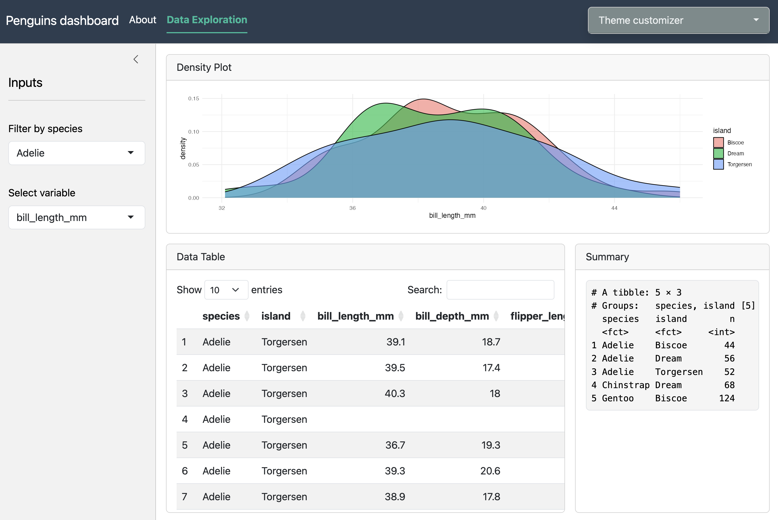
The use of theme presets or custom-defined themes are applied to all major components of the app’s UI, with the most notable exception being plots. While the font styles and theme colors are impacted by the specified theme that was provided, this is not easily applied to plots (such as those created using {ggplot2}) since they are rendered separately. However, we can achieve this consistent styling across the entire Shiny app (including plots!) using the {thematic} package. By simply adding thematic_shiny() outside of the UI and server components, this will update the color palettes used by the provided theme. To ensure that the selected fonts are also applied to the plot, you need to specify font = "auto" as an argument within this function. It is also generally good practice to load the {showtext} R package, which also helps with handling fonts when using {thematic}. An example is shown below:
library(shiny)
library(bslib)
library(thematic)
library(showtext)


thematic_shiny(font = 'auto')  #make theme for ggplot2 consistent w/ app

ui <- page_navbar(
  ...
)
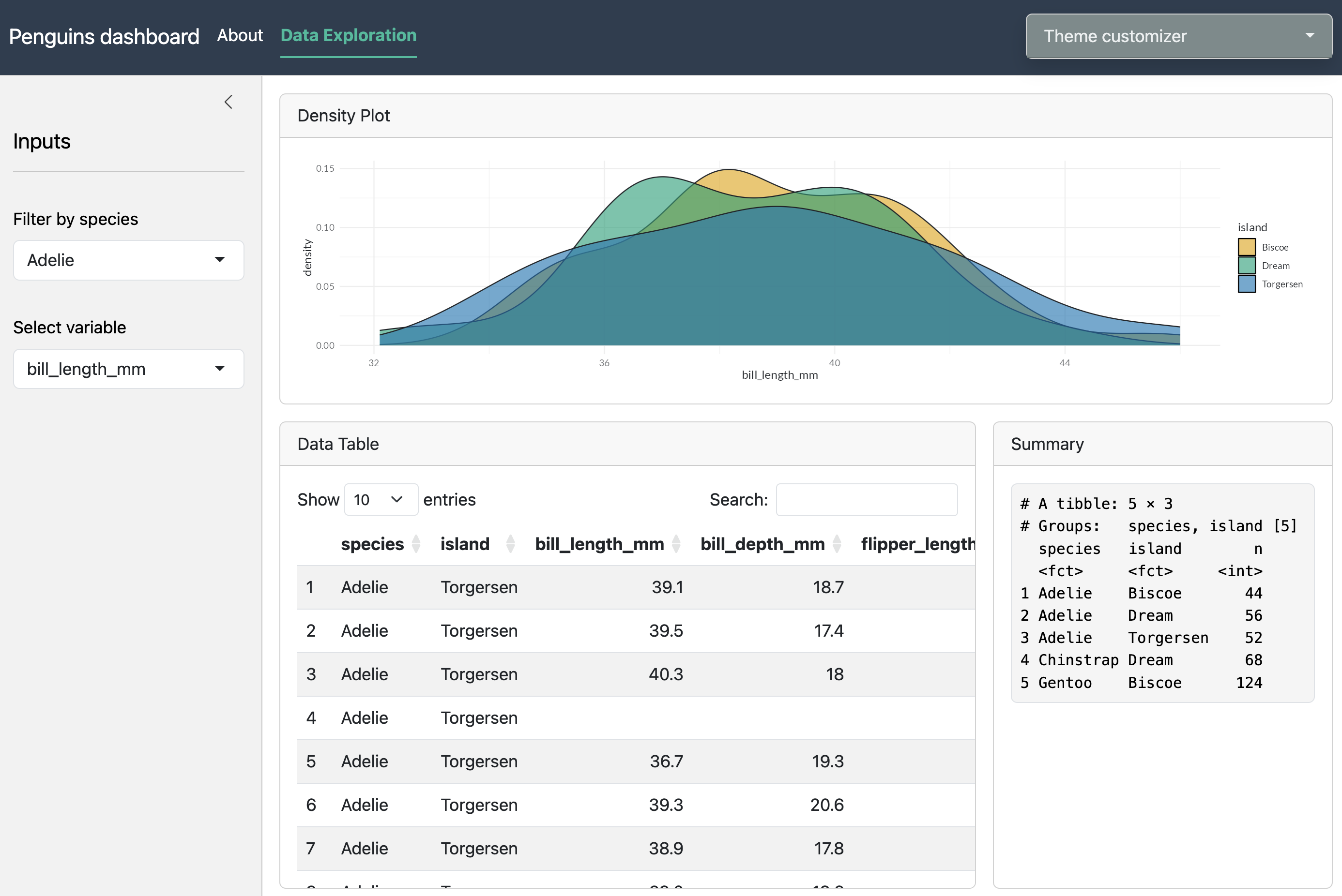
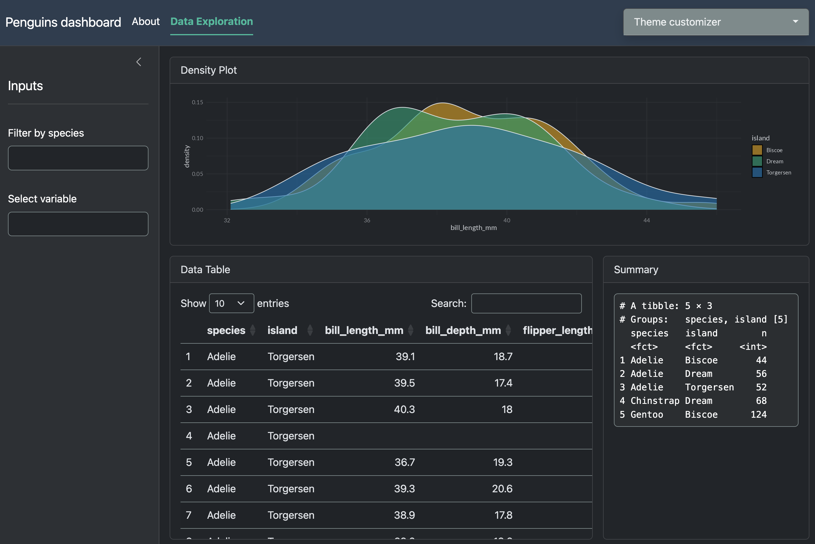
As compared to the screenshot above that used the “flatly” theme without using {thematic}, the below screenshots show examples of “flatly” when automatic theming with {thematic} is used, as well as an example when using a dark-mode theme. You can see that the fill colors for the density plot match the theme, and even the background of the plot is changed to black automatically without needing to adjust any {ggplot2} code.


Additional information on custom theming for Shiny apps can be found at the webpages for bslib and thematic.
Exercise 1
library(palmerpenguins)
library(ggplot2)
library(dplyr)
library(shiny)
library(bslib)
library(DT)
library(thematic)
library(showtext)


#################
### Define UI ###
#################


ui <- page_navbar(
  title = "Penguins dashboard",

  # Move navbar tabs to be right-aligned
  nav_spacer(),

  # First page
  nav_panel(
    title = "About",

    # Title for text body
    h1("Palmer penguins"),

    # First paragraph of text
    p("Data were collected and made available by Dr. Kristen Gorman and the Palmer Station, Antarctica LTER, a member of the Long Term Ecological Research Network."),

    # Second paragraph of text
    p("The {palmerpenguins} package contains two datasets. Both datasets contain data for 344 penguins. There are 3 different species of penguins in this dataset, collected from 3 islands in the Palmer Archipelago, Antarctica. More info can be found at this link:"),

    # Link to {palmerpenguins} package website
    a("https://allisonhorst.github.io/palmerpenguins/", href = "https://allisonhorst.github.io/palmerpenguins/"),

    # Artwork from Allison Horst
    img(src = "https://allisonhorst.github.io/palmerpenguins/reference/figures/lter_penguins.png")
  ),


  # Second page
  nav_panel(
    title = "Data Exploration",

    # Content for page
    layout_sidebar(
      # Define sidebar inputs
      sidebar = sidebar(
        title = "Inputs",

        # Filter data by species
        selectInput(
          inputId = "species",
          label = "Filter by species",
          choices = unique(penguins$species)
        ),

        #create dropdown selection for numeric columns
        varSelectInput(
          inputId = "var",
          label = "Select variable",
          data = dplyr::select_if(penguins, is.numeric)
        ),
      ),  #close sidebar

      # Main panel content
      layout_columns(
        col_widths = c(12, 8, 4),
        row_heights = c(2, 3),

        # Density plot
        card(
          card_header("Density Plot"),
          plotOutput("dens"),
          full_screen = TRUE
        ),

        # Table
        card(
          card_header("Data Table"),
          DT::dataTableOutput("tbl"),
          full_screen = TRUE
        ),

        # Text
        card(
          card_header("Summary"),
          verbatimTextOutput("txt"),
          full_screen = TRUE
        )
      )
    )
  ),

  # Add dark/light mode switch to navbar
  nav_item(input_dark_mode())

)


#####################
### Define server ###
#####################

server <- function(input, output, session) {


  # Create reactive object
  penguins_react <- reactive({
    penguins |>
      filter(species == input$species)
  })

  # Create density plot based on selection from inputs
  output$dens <- renderPlot({
    ggplot(penguins_react()) +
      geom_density(aes(!!input$var, fill = island), alpha = 0.6)
  })


  # Create interactive table via {DT}
  output$tbl <- DT::renderDataTable(
    datatable(
      data = penguins_react()
    )
  )


  # Summarize penguins dataset for text
  output$txt <- renderPrint({
    penguins |>
      group_by(species, island) |>
      count()
  })


}


###############
### Run app ###
###############

shinyApp(ui, server)
Using the included code:
- Choose a preset Bootswatch theme you prefer and apply to the app
- Set the base font to ‘Nunito Sans’ (Google), heading font to ‘Montserrat’ (Google), and code font to ‘Courier New’
- Change primary accent color to “#E69F00”
- Ensure that theme is also applied to
ggplot2figure
library(palmerpenguins)
library(ggplot2)
library(dplyr)
library(shiny)
library(bslib)
library(DT)
library(thematic)
library(showtext)


#################
### Define UI ###
#################

thematic_shiny(font = "auto")

ui <- page_navbar(
  title = "Penguins dashboard",
  theme = bs_theme(bootswatch = "pulse",
                   base_font = font_google('Nunito Sans'),
                   heading_font = font_google('Montserrat'),
                   code_font = "Courier New",
                   primary = "#E69F00"),

  # Move navbar tabs to be right-aligned
  nav_spacer(),

  # First page
  nav_panel(
    title = "About",

    # Title for text body
    h1("Palmer penguins"),

    # First paragraph of text
    p("Data were collected and made available by Dr. Kristen Gorman and the Palmer Station, Antarctica LTER, a member of the Long Term Ecological Research Network."),

    # Second paragraph of text
    p("The {palmerpenguins} package contains two datasets. Both datasets contain data for 344 penguins. There are 3 different species of penguins in this dataset, collected from 3 islands in the Palmer Archipelago, Antarctica. More info can be found at this link:"),

    # Link to {palmerpenguins} package website
    a("https://allisonhorst.github.io/palmerpenguins/", href = "https://allisonhorst.github.io/palmerpenguins/"),

    # Artwork from Allison Horst
    img(src = "https://allisonhorst.github.io/palmerpenguins/reference/figures/lter_penguins.png")
  ),


  # Second page
  nav_panel(
    title = "Data Exploration",

    # Content for page
    layout_sidebar(
      # Define sidebar inputs
      sidebar = sidebar(
        title = "Inputs",

        # Filter data by species
        selectInput(
          inputId = "species",
          label = "Filter by species",
          choices = unique(penguins$species)
        ),

        #create dropdown selection for numeric columns
        varSelectInput(
          inputId = "var",
          label = "Select variable",
          data = dplyr::select_if(penguins, is.numeric)
        ),
      ),  #close sidebar

      # Main panel content
      layout_columns(
        col_widths = c(12, 8, 4),
        row_heights = c(2, 3),

        # Density plot
        card(
          card_header("Density Plot"),
          plotOutput("dens"),
          full_screen = TRUE
        ),

        # Table
        card(
          card_header("Data Table"),
          DT::dataTableOutput("tbl"),
          full_screen = TRUE
        ),

        # Text
        card(
          card_header("Summary"),
          verbatimTextOutput("txt"),
          full_screen = TRUE
        )
      )
    )
  ),

  # Add dark/light mode switch to navbar
  nav_item(input_dark_mode())

)


#####################
### Define server ###
#####################

server <- function(input, output, session) {


  # Create reactive object
  penguins_react <- reactive({
    penguins |>
      filter(species == input$species)
  })

  # Create density plot based on selection from inputs
  output$dens <- renderPlot({
    ggplot(penguins_react()) +
      geom_density(aes(!!input$var, fill = island), alpha = 0.6)
  })


  # Create interactive table via {DT}
  output$tbl <- DT::renderDataTable(
    datatable(
      data = penguins_react()
    )
  )


  # Summarize penguins dataset for text
  output$txt <- renderPrint({
    penguins |>
      group_by(species, island) |>
      count()
  })


}


###############
### Run app ###
###############

shinyApp(ui, server)